Tutorial 1: 10X Visium DLPFC dataset
In this tutorial, we show how to apply scSTADE to identify spatial domains on 10X Visium data. As a example, we analyse the 151672 sample of the dorsolateral prefrontal cortex (DLPFC) dataset.
The source code package is freely available at https://github.com/cuiyaxuan/scSTADE/tree/master. The datasets used in this study can be found at https://drive.google.com/drive/folders/1H-ymfCqlDR1wpMRX-bCewAjG5nOrIF51?usp=sharing.
First, cd /home/.../scSTADE/scSTADE_Cluster_Functions/
# Using python virtual environment with conda. Please create a Pytorch environment, install Pytorch and some other packages, such as "numpy","pandas", "scikit-learn" and "scanpy". See the requirements.txt file for an overview of the packages in the environment we used to produce our results. Alternatively, you can install the environment dependencies in the following sequence to minimize environment conflicts.

conda create -n pipeline
source activate pipeline

conda search r-base
conda install r-base=4.2.0
conda install python=3.8

conda install conda-forge::gmp
conda install conda-forge::r-seurat==4.4.0
conda install conda-forge::r-hdf5r
conda install bioconda::bioconductor-sc3

conda install conda-forge::pot
conda install pytorch torchvision torchaudio pytorch-cuda=11.8 -c pytorch -c nvidia
conda search -c conda-forge r-mclust
conda install -n pipeline -c conda-forge r-mclust=5.4.10

pip install scanpy
pip install anndata==0.8.0
pip install pandas==1.4.2

conda install -c conda-forge rpy2=3.5.1
pip install scikit-learn==1.1.1
pip install scipy==1.8.1
pip install tqdm==4.64.0
pip install scikit-misc
to install some R packages.
import rpy2.robjects as robjects
robjects.r('''
install.packages('foreach')
install.packages('doParallel')
           ''')
import sys
sys.path.append("/.../scSTADE-master/scSTADE_Cluster_Functions")
# Input the path.
from scSTADE import scSTADE
import os
import torch
import pandas as pd
import scanpy as sc
from sklearn import metrics
import multiprocessing as mp
import dropout

file = '/home/cuiyaxuan/spatialLIBD/151672' # Input the data path for the nonlinear model.
count='151672_filtered_feature_bc_matrix.h5' # Input the file name for the nonlinear model.
adata = sc.read_visium(file, count_file=count, load_images=True)

dropout.setup_seed(41)
dropout_rate=dropout.dropout(adata)
print(dropout_rate) # Data quality assessment.

device = torch.device('cuda:0' if torch.cuda.is_available() else 'cpu') # cpu or gpu
n_clusters = 5  # Users can input either the default number of clusters or the estimated number of clusters.


import rpy2.robjects as robjects

data_path = '/home/cuiyaxuan/spatialLIBD/151672/151672_filtered_feature_bc_matrix.h5' # Input the data path and file name for the nonlinear model.
position_path = '/home/cuiyaxuan/spatialLIBD/151672/spatial/tissue_positions_list.csv' # Input the data path and position file name for the nonlinear model.
ARI_compare='/home/cuiyaxuan/spatialLIBD/151672/cluster_labels_151672.csv' #  Input the ground truth data path and file name for comparing with the clustering results

robjects.globalenv['data_path'] = robjects.vectors.StrVector([data_path])
robjects.globalenv['position_path'] = robjects.vectors.StrVector([position_path])
robjects.globalenv['ARI_compare'] = robjects.vectors.StrVector([ARI_compare])
robjects.globalenv['n_clusters'] = robjects.IntVector([n_clusters])


#The ARI accuracy and clustering labels have been generated and saved as CSV files.
if dropout_rate>0.85:
   for i in [4000, 4500, 5000]:
      file_fold = file
      adata = sc.read_visium(file_fold, count_file = count, load_images=True)
      adata.var_names_make_unique()
      model = scSTADE(adata,device=device,n_top_genes=i)
      adata = model.train()
      radius = 50
      tool = 'mclust' # mclust, leiden, and louvain
      from utils import clustering

      if tool == 'mclust':
         clustering(adata, n_clusters, radius=radius, method=tool, refinement=True) # For DLPFC dataset, we use optional refinement step.
      elif tool in ['leiden', 'louvain']:
         clustering(adata, n_clusters, radius=radius, method=tool, start=0.1, end=2.0, increment=0.01, refinement=False)

      adata.obs['domain']
      adata.obs['domain'].to_csv(f"label_{i}.csv")


   robjects.r('''
   library(SingleCellExperiment)
   library(SC3)
   library("Seurat")
   library("dplyr")
   library("hdf5r")
   library(foreach)
   library(doParallel)


   print(data_path)
   print(position_path)
   print(ARI_compare)
   print(n_clusters)

   source('Cri4.R')
   hc1= Read10X_h5(data_path) #### to your path and project name
   feature<-select_feature(hc1,4000,500)
   detectCores()
   cl <- makeCluster(3) # call 3 cpu cores
   k=n_clusters # k represent the number of spatial domains.
   parLapply(cl,1:3,feature=feature,k=k,pearson_metric)
   stopCluster(cl)

   tissue_local=read.csv(position_path,row.names = 1,header = FALSE)
   adj_matrix=construct_adj_matrix(feature[[1]],tissue_local)
   write.table(adj_matrix,file="adj_matrix.txt",sep=" ",quote=TRUE)
   detectCores()
   cl <- makeCluster(3) # call 3 cpu cores
   parLapply(cl,1:3,K=k,spectral_nei)
   stopCluster(cl)


   source('GNN_Tradition_6.R')

   source('label_ARI.R')
   true_label=read.csv(ARI_compare,row.names = 1)
   conlabel(hc1,k,true_label,compare=T)        ####   compare=T is compare ARI with the ground truth, compare=F is no compare ARI with the ground truth. Writing ARI results to a CSV file.
            ''')
else:

   file_fold = file
   adata = sc.read_visium(file_fold, count_file= count, load_images=True)
   adata.var_names_make_unique()
   model = scSTADE(adata,device=device,n_top_genes=5000)
   adata = model.train()
   radius = 50
   tool = 'mclust' # mclust, leiden, and louvain
   from utils import clustering

   if tool == 'mclust':
      clustering(adata, n_clusters, radius=radius, method=tool, refinement=True) # For DLPFC dataset, we use optional refinement step.
   elif tool in ['leiden', 'louvain']:
      clustering(adata, n_clusters, radius=radius, method=tool, start=0.1, end=2.0, increment=0.01, refinement=False)

   adata.obs['domain']
   adata.obs['domain'].to_csv(f"label.csv")
0.8968134495641344
0.8968134495641344
Begin to train ST data...
0%| | 0/500 [00:00<?, ?it/s]
0
0%| | 1/500 [00:02<24:55, 3.00s/it]
0
0%|▏ | 2/500 [00:05<23:31, 2.83s/it]
0
1%|▎ | 3/500 [00:08<22:00, 2.66s/it]
0
1%|▎ | 4/500 [00:11<23:22, 2.83s/it]
0
1%|▍ | 5/500 [00:14<23:54, 2.90s/it]
0
1%|▌ | 6/500 [00:17<24:44, 3.00s/it]
0
1%|▌ | 7/500 [00:20<25:19, 3.08s/it]
0
2%|▋ | 8/500 [00:23<24:59, 3.05s/it]
0
2%|▊ | 10/500 [00:29<25:01, 3.06s/it]
0
2%|▉ | 11/500 [00:32<24:55, 3.06s/it]
0
2%|█ | 12/500 [00:35<24:35, 3.02s/it]
100%|█████████████████████████████████████████| 500/500 [30:28<00:00, 3.66s/it]
Optimization finished for ST data!
fitting ...
  |======================================================================| 100%
[1] "/home/cuiyaxuan/spatialLIBD/151672/151672_filtered_feature_bc_matrix.h5"
[1] "/home/cuiyaxuan/spatialLIBD/151672/spatial/tissue_positions_list.csv"
[1] "/home/cuiyaxuan/spatialLIBD/151672/cluster_labels_151672.csv"
[1] 5
R[write to console]: Calculating gene variances
R[write to console]:

R[write to console]: 0%   10   20   30   40   50   60   70   80   90   100%

R[write to console]: [----|----|----|----|----|----|----|----|----|----|
loaded SC3 and set parent environment
 要求されたパッケージ foreach をロード中です
 要求されたパッケージ rngtools をロード中です
loaded SC3 and set parent environment
 要求されたパッケージ foreach をロード中です
 要求されたパッケージ rngtools をロード中です
|============================================== | 65%
starting worker pid=3761761 on localhost:11781 at 13:11:26.174
 要求されたパッケージ SC3 をロード中です
loaded SC3 and set parent environment
 要求されたパッケージ foreach をロード中です
 要求されたパッケージ rngtools をロード中です
 警告メッセージ:
 パッケージ ‘SC3’ はバージョン 4.2.3 の R の下で造られました
 警告メッセージ:
 パッケージ ‘SC3’ はバージョン 4.2.3 の R の下で造られました
 警告メッセージ:
 パッケージ ‘SC3’ はバージョン 4.2.3 の R の下で造られました
R[write to console]: Calculating gene variances
R[write to console]:

R[write to console]: 0%   10   20   30   40   50   60   70   80   90   100%

R[write to console]: [----|----|----|----|----|----|----|----|----|----|


R[write to console]: *
R[write to console]: *
R[write to console]: *
R[write to console]: *
R[write to console]: *
R[write to console]: *
R[write to console]: *
R[write to console]: *
R[write to console]: *
R[write to console]: |
import matplotlib as mpl
import scanpy as sc
import numpy as np
import pandas as pd
import seaborn as sns
import matplotlib.pyplot as plt
import warnings
import visual
mpl.rcParams['pdf.fonttype'] = 42
mpl.rcParams["font.sans-serif"] = "Arial"
warnings.filterwarnings('ignore')
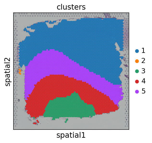
file_fold = '/home/cuiyaxuan/spatialLIBD/151672/' # your path
adata = sc.read_visium(file_fold, count_file='151672_filtered_feature_bc_matrix.h5', load_images=True)
df_label=pd.read_csv('./label.csv', index_col=0)
#df_label=pd.read_csv('./label_5000.csv', index_col=0) ##If the dropout rate is less than 0.85, visualize the data using "label_5000.csv".
visual.visual(adata,df_label)
#cells after MT filter: 4015

WARNING: saving figure to file figures/showvisualdomainplot_plot.pdf